When scientists (again, I should really limit myself to astrophysicists, because I cannot really speak for other sciences) need to create figures to put in journal papers, in presentations or on posters, they usually need to create plots: graphs with an x and y axis and lines and dots, contours, colour maps… There are many tools you can use for this, and astrophysicists usually fall back to either Python’s matplotlib or licensed software like IDL to do this.

Sometimes however, the required figures are not plots. When you are working in scientific computing, you might want to illustrate an algorithm or concept, and then things like flowcharts or simple diagrams come into play. While traditional plotting tools (certainly matplotlib) can be used for this purpose when you tweak them enough (a painful and slow process), there are much better tools available. These tools are not only more suited for the task at hand, but also a lot more powerful.

In this post I want to give a brief introduction to one of these tools, called TikZ. TikZ is not really a tool, but is a language package that is part of LaTeX, and that can be used to generate vector graphics that can be directly included in .pdf-documents generated with LaTeX. Since astrophysicists as myself use LaTeX all the time, this makes it a very accessible tool.

How does it work?

As with any LaTeX package, the only requirement to start using TikZ inside a document is by including the corresponding package in the preamble of your document:

\usepackage{tikz}

Depending on your LaTeX installation, you might need to install the TikZ package first, but as with any other LaTeX package this should be very easy.

Once included, you can add a diagram or flowchart anywhere in your document by putting it in a tikzpicture environment:

\begin{tikzpicture}

\end{tikzpicture}

Let’s start with a minimal example LaTeX-file:

\documentclass[12pt]{article}
\usepackage{tikz}

\begin{document}

\begin{tikzpicture}
\draw (0.0, 0.0) -- (1.0, 1.0);
\end{tikzpicture}

\end{document}

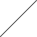
If you save this as a .tex-file and then compile this with pdflatex, the resulting .pdf-document should contain a single, non-impressive line:

The command to draw this line is reasonably self-explanatory: we want to draw a line, from coordinate (0.0, 0.0) to (1.0, 1.0), and this line has to be straight (--). Just as some programming languages, TikZ also requires you to put a ; at the end of each line. \draw starts the command, and ; concludes it. This is the general way commands in TikZ work. I will introduce other commands later in this post.

By default, TikZ will use a length unit of 1.0 cm for all coordinates and distances. You can change this default by providing an additional argument to the tikzpicture environment, e.g.

\begin{tikzpicture}[x = 2.0cm, y = 3.0cm]

will set the horizontal and vertical length unit to respectively 2.0 cm and 3.0 cm.

Standalone figures

The example above shows you how to include basic drawings straight into your .pdf-document. Sometimes however, it can be useful to generate images on their own, e.g. as a .png-file. You could of course generate a .pdf-document containing your image and then convert this into an image using tools like convert (part of ImageMagick), but this is quite involved. Fortunately, LaTeX has a way of doing this for you, in the form of the standalone package.

To generate the example above as a .png-image instead of a .pdf-document, simply replace the first line with

\documentclass[convert={density=300,outext=.png}]{standalone}

Again, you might need to install standalone using your LaTeX package manager first. The convert= option tells standalone to use ImageMagick’s convert to convert the result into an image with the given output extension (outext=.png), and with the given resolution of 300 dpi (density=300). standalone will automatically make sure the size of the document is adapted to that of the visible content.

To compile the image, run

pdflatex -shell-escape <name of .tex file>

instead of the usual pdflatex command. The -shell-escape argument is required to enable standalone to invoke the convert command. pdflatex will then generate a .png-image containing your image (this is exactly how the example images in this post were made).

Note that on recent versions of Ubuntu (16.04 and higher), the default security settings of ImageMagick prevent convert from opening .pdf-documents, so that the command above will fail to produce a .png-file. To remedy this, you need to manually disable the rule in /etc/ImageMagick-6/policy.xml that prevents ImageMagick from reading .pdf-files. Open the file and comment out this line

 <policy domain="coder" rights="none" pattern="PDF" />

See this post on Ask Ubuntu.

Diagrams and flowcharts

So far, I have only shown you how to draw a simple line and generate a .png-image using pdflatex. However, much of the power of TikZ comes from its close ties with LaTeX, allowing you to embed LaTeX text into images, e.g. to generate a flowchart or a drawing with annotations.

To add text in TikZ, you need to define a node. This can be done in various ways, but the usual way to do this is by using a \node command:

\node(label)[properties] at (0.0, 0.0) {This is a node};

Let me break this down for you. First of all, \node is the command you want TikZ to perform: defining a node. (label) is what it says: this defines a label that will be attached to this node. The label is not visible, but can be used to refer to this node in subsequent TikZ commands. [properties] contains the properties of the node. Using properties, you can change about every aspect of the node, e.g. its colour, size, bounding box, position… I will show some of these properties at work later. at (0.0, 0.0) defines the location of the node (in the TikZ internal length units). {This is a node} is the caption of the node, this is the text that will be displayed in the image. This text is rendered with LaTeX, and can contain any allowed LaTeX command (including additional tikzpicture environments!). It inherits the text properties (font, font size…) of the document. By default, the text is centred within the node; the node automatically adjusts its size to fit the caption.

Except for the \node command, all other instructions are optional; by default the node is placed at the origin of the coordinate system, has no label, and is empty. If you only want to use nodes and you only care about their relative position, you can position the nodes using their properties, e.g.

\begin{tikzpicture}[node distance=2.0cm]
\node(a)[rectangle, draw=black] {$a$};
\node(b)[rectangle, draw=red, right of=a] {$b$};
\draw[->] (a) -- (b);
\end{tikzpicture}

will put the b-node to the right of the a-node, at a default distance of 2.0cm:

The \draw[->] (a) -- (b); command creates a line joining the two nodes (using the node labels) with an arrow at the end of the line.

Finally, you can also create nodes as part of other commands:

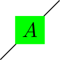
\draw (0.0, 0.0) --node[fill=green]{$A$} (1.0, 1.0);

This will automatically centre the node on the line drawn by the \draw command:

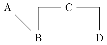
Once you know how to create nodes and join them using appropriate draws, you have almost everything you need to create flowcharts. One additional thing you might need to know is how to use the -- in the \draw command:

\node(a) {A};
\node(b) [right of=a, below of=a] {B};
\node(c) [right of=b, above of=b] {C};
\node(d) [right of=c, below of=c] {D};
\draw (a) -- (b);
\draw (b) |- (c);
\draw (c) -| (d);

Notice how the various \draw commands result in different orientations for the node connections:

Note that while TikZ is very powerful in creating flowcharts, it is not very good at helping you figure out how to optimally position your nodes. There are other tools (e.g. Graphviz] that can do this for you. On Linux systems, there is a utility tool called dot2tex that can convert a Graphviz .dot-file into a properly positioned TikZ flowchart:

dot2tex -f tikz -t raw --figonly <input .dot file> > <output .tex file>

Embedding TikZ into LaTeX figures

In the first example above, you already saw how to embed a tikzpicture into a .pdf-document. This example however did not give you any control over the size and position of the drawing: it was simply placed at the current position in the document, and the size was determined by the size of the drawing. This situation is pretty much equivalent to including a figure using \includegraphics without any size options.

Just as with figures, you can significantly improve the positioning of a tikzpicture by wrapping it into a figure environment:

\begin{figure}
\begin{tikzpicture}
...
\end{tikzpicture}
\end{figure}

This way, you can treat the drawing as if it was any other figure (including captions and labels), but the figure itself will still inherit the text properties from your main document, and determine its own size. You can make the document a bit more tidy by putting the TikZ code into a separate .tex-file and including that using \input.

If you want to control the figure size yourself, you have to put the TikZ code into a separate file and wrap the \input command in a resizebox, like this:

\begin{figure}
\resizebox{0.5\textwidth]{!}{\input{tikz_source.tex}}
\end{figure}

Note that this means the TikZ figure does no longer inherit the font size of the main document.

TiKZ language reference

So far, I have just illustrated some of the available TikZ commands and options and a full reference is far beyond the scope of this post. http://www.texample.net/tikz/examples/ hosts a large set of TikZ examples, and https://en.wikibooks.org/wiki/LaTeX/PGF/TikZ is also a very good source of information if you want to know more about basic TikZ commands. Let me just mention some important aspects that might point you in the right direction for specific use cases:

• apart from \draw, there are also \fill and \filldraw commands. The difference between these is the way they apply colour to the objects they draw: \draw generates lines and only colours those, \fill generates a contour and then colours the inside of that contour, filldraw first draws the contour and then fills it as well. \shade is an alternative for \fill that uses a gradient fill.
• you can generate specific shapes by passing keywords to \draw (or \fill(draw)): \draw (0.0, 0.0) circle (0.5); for example creates a circle centred on (0.0, 0.0) with radius 0.5. There are also commands for rectangles, arcs, ellipses, parabolas, sine waves… So it is worth checking if your specific shape already exists before starting to define it line by line.
• you can create labelled property groups that can be reused for multiple commands. This is very helpful if you e.g. want to create a specific style for the nodes in a flowchart, and then apply to that all nodes. To do this, add a \tikzstyle{name} = [properties] line to the preamble of your LaTeX document, and then simply add the name as a property to the element you want to give this style.
• similarly, you define your own colours using a \definecolor command in the preamble and then reuse these for multiple TikZ elements.
• to reuse a specific drawing command, you can define your own LaTeX commands in the preamble of your document and then use them inside your TikZ code.
• TikZ has a large number of additional libraries that help you create more powerful figures. You can activate these using the \usetikzlibrary command in the preamble of your document.

Cover image

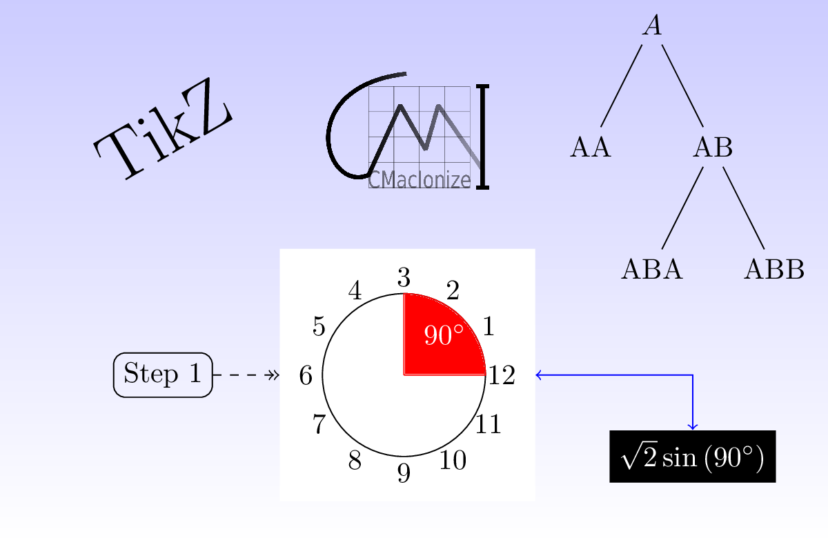
To conclude, here is the full source of the cover image of this post, that includes a lot of useful commands and properties:

\documentclass[convert={size=1200x800,outext=.png}]{standalone}
\usepackage{tikz}
\begin{document}
\begin{tikzpicture}

% background rectangle
\shade[top color=blue!20, bottom color=white] (0.0, 0.0) rectangle (10.16, 6.6);

% a simple text node
\node(startnode)[draw = black, rounded corners] at (2.0, 2.0) {Step 1};

% tikzception: a TikZ picture within a node!
\node(circlenode)[fill = white] at (5.0, 2.0) {\begin{tikzpicture}
% a circle
\draw (0.0, 0.0) circle (1.0);
% a quarter of the circle, using an arc
\filldraw[color = red] (0.0, 0.0) -- (1.0, 0.0) arc (0:90:1.0) -- (0.0, 0.0);
% a label for the quarter
\node[color = white] at (0.5, 0.5) {$90^\circ{}$};
% labels for the circle
\foreach \a in {1,2,...,12}{
\draw (\a*360/12: 1.2) node{\a};
}
\end{tikzpicture}};

% node with equation and fill and text colours
\node(equationnode)[fill = black, text = white] at (8.5, 1.0)
  {$\sqrt{2}\sin{}(90^{\circ{}})$};

% flowchart connections
\draw[->>, dashed] (startnode) -- (circlenode);
\draw[<->, color = blue] (circlenode) -| (equationnode);

% a tree
\node at (8.0, 6.3) {$A$}
  child {node {AA}}
  child {node {AB}
    child {node {ABA}}
    child {node {ABB}}};

% Title node. Larger font and rotated
\node[rotate = 30] at (2.0, 5.0) {\Huge{}TikZ};

% Node with embedded external image
\node at (5.0, 5.0) {\includegraphics[width=2.0cm]{logo.png}};

\end{tikzpicture}
\end{document}