Space-filling curves
One of the perks or issues of being a researcher (pick your favourite) is that what you do does not necessarily always result in something useful. You could of course argue semantics and ask yourself what is useful? (definitely if you are an astronomer and think about your field), but I think it is easy to answer that question from a personal point of view: something useful is something that gives you the feeling that it was worth it.
The topic of this post is one of these things that I spent a lot of time on at some point (during my PhD, when I could afford such extravagances), but that in hindsight was not useful. Interesting, but definitely not useful. This post is an attempt to maybe make it useful after all, by at least sharing what I know and what I figured out. And by then explaining why you should definitely (not) spend time on this same topic.
The topic of this post are space-filling curves. These are geometrical constructs that almost automatically show up whenever you are breaking down space into regular blocks, and are very easy to work with or think about when you are dealing with bit series. And they are in a way incredibly beautiful and elegant. But definitely not as useful as I thought they were. Here is a short introduction.
What are space-filling curves?
Space-filling curves are, as the name says, curves that fill space. This means that if you define a space (for example a square), then a space-filling curve in that space is a single curve that moves through every point of that space, without ever visiting the same point twice. Of course, this only works if the square (or more generally, the space) is a finite space, i.e. has a finite number of points in it. Or at least has a countable number of points in it. Let’s not be too mathematical about this; I will only ever consider finite spaces.
The square space could for example only consist of 4 points: the midpoints of the 4 smaller squares you get when you subdivide the square into 4 equal parts. In this case, a space filling curve could look like this:

Or like this:
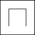
The two curves above are both level 1 space-filling curves, since they fill the space that you get by subdividing the square once into 4 equal smaller squares. The first one is what we call a Morton or Z-order space-filling curve (N-order would have been better, unless you tilt your head), the second is what we call a Hilbert curve. You can already see the difference between both curves: while the Morton curve just traverses the space column by column, the Hilbert curve has a twist in it. As a result, the distance between successive points in the Hilbert curve is always the same, while for the Morton curve it is not. This distinction remains for higher level curves.
If we subdivide the square again (we subdivide each smaller square into 4 equal even smaller squares), we end up with a level 2 subdivision, in which we can define level 2 space-filling Morton and Hilbert curves:

For the Morton curve, it is immediately clear what we do: we just copy the original level 1 Morton curve into each level 1 square, and then order these along the original level 1 curve to make up the total curve. When we reach the end of the second level 1 square, we need to jump to the third level 1 square.
For the Hilbert curve, things are a bit more complicated. The level 1 squares also contain a copy of the level 1 curve, but unlike for the Morton curve, this copy is rotated, so that the endpoint of each level 1 square matches the starting point of the next square along the level 1 ordering. By doing this, we guarantee that the level 2 curve still satisfies the property that the distance between successive points is always the same. Notice that the rotations for the different squares are different and depend on the position of that square along the level 1 curve.
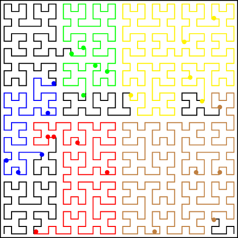
Once we know how to go from a level 1 to a level 2 space-filling curve, we know everything we need to move to even higher levels. Here are some level 5 space-filling curves:

You can see that the curves indeed start to fill the entire square. A curve with a high enough level should be able to fill any finite space.
Why are space-filling curves useful?
One of the main reasons I ever started looking into space-filling curves is because of their use in spatial domain-decomposition. Imagine that you have a large number of points that are somewhat arbitrarily ordered in our square space, like this:
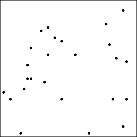
Spatial domain-decomposition deals with the following question: what is the best way to divide this set of points into an arbitrary number of groups, so that points in the same group are guaranteed to be close to each other? You might notice that this question is not formulated very rigorously. I will come back to that later (spoiler: it is one of the reasons space-filling curves are not that useful).
Before answering this question, let me first explain why a scientist (and more importantly: an astronomer!) would even ask such a question. The reason for this are large (N-body) simulations. Just imagine that the points above are stars in a cluster, and that you want to compute the gravitational forces that act on these stars. In principle, to compute these forces, you would need to loop over the stars, one by one, and for each of them compute the gravitational interaction between that star and every other star in the cluster. If you have stars, then the computation for every star would involve other stars, and you would have computations in total. For the specific example shown above, this is not too bad. But things get a bit tricky if gets very big…
They get tricky for two reasons: (1) the number of computations grows really fast as gets bigger, (2) if gets really big, the stars might no longer fit on a single computer. This might sound very unlikely, but actually happens a lot these days, as large N-body simulations can go up to !
To deal with the growing number of computations, astrophysicists have developed clever algorithms. They realised for example that the force for a given star is usually dominated by close neighbours of that star, and that the forces due to stars that are further away can be approximated reasonably accurately by grouping them together, drastically decreasing the number of computations per star. To deal with too big to fit on a single computer, they started using parallel computers that consist of many computers linked together. Each computer stores only a fraction of the stars, and sends information about these to the other computers when necessary.
Now we get back to the original point, because to divide the stars among the different computers, we need to perform a spatial domain-decomposition: we want to make sure that all computers have roughly the same number of stars (the same number of computations), but we also want to make sure that stars that are close together are generally found on the same computer, because that reduces the amount of communication necessary during the computation.
And now for the answer: what we could try to do is fit a space-filling curve through the stars (let’s revert to calling them points). This will effectively map the 2D distribution of points onto a 1D line, so that we can assign a unique number to each point that we can compare with other points to sort them. Additionally, we know that points that are close on the space-filling curve are generally also close in space (especially for the Hilbert curve). If we know cut up the space-filling curve into (almost) equal pieces, we accomplish the desired spatial decomposition:
More about this later…
How do we compute space-filling curves?
As I mentioned before, space-filling curves are inherently linked to a level of subdivision of the space in which they are defined. This level defines the number of points in the space, and also tells you how far you have to go down when constructing the curve.
To compute a space-filling curve, we hence need to discretise our space to some level. The easiest way to do this is by mapping the coordinates of all points in the space to integer values with a fixed number of bits, say . If we are in a square space with side length , then the integer coordinates for a point with coordinates are
Note that if , then this guarantees , so the integer coordinates will exactly fit in an integer value with bit precision.
Both the Morton and the Hilbert space-filling curve can then be computed by using these integer coordinates and mapping them to an integer key with bits. The key encodes the order of the points along the space-filling curve, and the space-filling curve can be generated by sorting the points on the key and the drawing the connections between the point in that order. This is exactly how the images above were made.
The difference between the Morton and Hilbert curves is the way their key is computed. For the Morton curve, the key, , is computed by interleaving the bits of and . This means that we run through the bit-wise representation of the two integer coordinates and one by one strip their bits and put them in the key. So if
and
then
We can understand this if we think about a single level of the curve, or hence a single bit of and and the 2 corresponding bits of . For the Morton curve, each level is equivalent, so this would be equivalent to a simple level 1 curve. For a level 1 curve, there would be 4 points in the space:
Now it is very easy to see that the (single) bit of tells us in which half of the square we are in the horizontal direction, while the same is true for in the vertical direction. The characteristic Z-shape (N-shape) of the Morton curve means that we want the to make up the lower part of the 2-bit key, while makes up the high part, so that we first traverse all the left vertical points and then all right ones.
Now suppose we were to move on to a level 2 curve. As we saw before, this curve follows the overall path of the level 1 curve, but has smaller copies of the curve for each of the points in the original curve. To make sure the key still follows the overall path of the level 1 curve, the level 1 key has to make up the highest part of the level 2 key. However, in (bit-wise) integer coordinates, the original level 1 points are now
since we added a level in our integer coordinate conversion formula and hence an additional factor 2 (which means we shift all bits 1 position to the left and add an extra 0-bit at the end). So the highest bit of the level 2 key is determined by the highest bits in the integer coordinates.
The new integer coordinates for the original level 1 curve points are each only 1 in 4 points for their specific smaller square, as the new 0-bit can be replaced by a 1-bit (and there are 4 available options). In fact, the situation is exactly the same as for the level 1 curve, so we can get the new low part of the level 2 key by doing the same we did for the level 1 key. And the same is true for higher level keys.
Because computing a Morton key only requires bit-wise operations, it can be done very efficiently on a computer. Below is a snippet of Python code that computes the Morton key for two integer coordinates x and y:
def get_morton_key(level, x, y):
  key = 0
  for i in range(level):
    key |= (x & 1) << (2 * i + 1)
    key |= (y & 1) << (2 * i)
    x >>= 1
    y >>= 1
  return key
What about the Hilbert curve?
Computing the Morton key simply requires you to interleave the bits of the integer coordinates of the points in your space. For the Hilbert key, things are a little bit more complicated. The reason for this are the twists in the Hilbert curve which require a rotation when going from one level to the next. Which means that the level 2 part of the Hilbert key can only be computed if you know what the level 1 part of the key is… Generally, the computation for the level key will depend on what happened on all higher levels (with lower values of ).
We could go through an awful lot of bit-wise geometry to derive bit-wise operations per level that would allow us to generate the Hilbert key in a similar fashion to the Morton key, i.e. by looping over the levels and performing some bit-wise magic on each of the levels to arrive at the right key bit for that level. We would then need to either rotate the key or rotate the integer coordinates from one level to the next, which involves even more bit-wise geometry. This is a very painful and slow process (and I know, because I’ve actually done it), and I will not go through it here.
We could also rethink the way we compute the keys. This is the method adopted by Jin & Mellor-Crummey (2005), the paper I eventually discovered during my space-filling curve exploration. Their idea is to use a lookup-table to compute keys for space-filling curves. The lookup-table acts as a sort of map, that tells you in which direction to move along the curve, starting from a given position. The easiest way to explain it is by using the Morton key as an example.
Let’s start again with the level 1 Morton curve. Instead of just drawing it however, we will now label the connections in the curve with the directions we need to move in to follow the curve between the different points, and we will label the points with the shape of the curve on the next level down (an inverse Z, since this will also be the Morton curve):
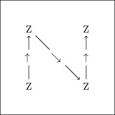
The entire curve can be described in terms of a simple map with the 1-bit integer coordinates as reference points:
- if the current integer position is , move up
- if the current integer position is , move down and right
- if the current integer position is , move up
- if the current integer position is , stop
We can also add directions for the next level to this map. These are very simple, since we know that the Morton curve looks the same on each level. But this will be useful for the Hilbert curve. The entire map can then be summarised as a simple table:
| map name | position 0 | position 1 | position 2 | position 3 |
|---|---|---|---|---|
| Z | (Z, ) | (Z, ) | (Z, ) | (Z, stop) |
The different elements in each column are respectively the name of the map on the next level and the movement direction that brings you to the next point on the current level.
To construct the key for a given set of coordinates, we need a slight variations on this table: we need to know which of the four corners of the square corresponds to which column in the map, because the number of that column is the bit we need to add to the Morton key on that level. Interestingly enough (and not surprising given what we saw before) we can get this number by interleaving the bits of the integer coordinates level by level. This is because the Morton curve itself gives us a unique way to order the four corners of a square.
Things are a bit different for the Hilbert curve, because there are 4 possible orientations of our curve that we can encounter, and hence 4 different maps (there are actually 8, because we can traverse all of these curves in reverse order):
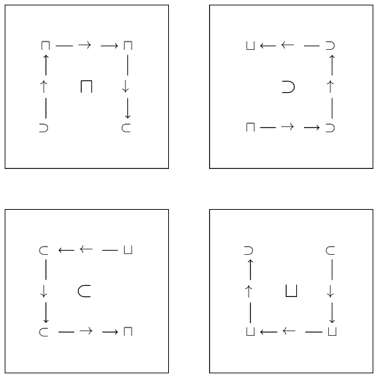
| map name | position 0 | position 1 | position 2 | position 3 |
|---|---|---|---|---|
| (, ) | (, ) | (, ) | (, stop) | |
| (, ) | (, ) | (, ) | (, stop) | |
| (, ) | (, ) | (, ) | (, stop) | |
| (, ) | (, ) | (, ) | (, stop) |
If this is not immediately clear, you can check this yourself by looking at the level 2 Hilbert curve above and following the direction of the curve. In this case we see why it makes sense to keep track of the direction and the map for the next level.
As before, we need a variant on this table to compute the Hilbert key. We can replace the arrows in the table above (we won’t need them) with the corresponding bit of the key (this is just the column number), and the rearrange the columns so that the four corners of the square are in Morton order:
| map name | position 0 | position 1 | position 2 | position 3 |
|---|---|---|---|---|
| (, 00) | (, 01) | (, 11) | (, 10) | |
| (, 00) | (, 11) | (, 01) | (, 10) | |
| (, 10) | (, 01) | (, 11) | (, 00) | |
| (, 10) | (, 11) | (, 01) | (, 00) |
The table is now all set to run our algorithm: we take the highest bits of the integer coordinates, and compute their level 1 Morton key. We then take the corresponding column of the -map. The key in that column is the key bit we need to add to this level of our Hilbert key. The map name in that column tells us which map to use for the next level. For the next level, we take the next two bits of the integer coordinates, compute their Morton key, and repeat the exercise, but now with the new map. The map information encodes all the rotations we need, so we don’t need to worry about any of this any more.
Here is a short snippet of Python code that computes the Hilbert key (note that the table in this script contains all 8 possible maps):
htable = np.array([
  [[7, 0], [0, 1], [6, 3], [0, 2]], [[1, 2], [7, 3], [1, 1], [6, 0]],
  [[2, 1], [2, 2], [4, 0], [5, 3]], [[4, 3], [5, 0], [3, 2], [3, 1]],
  [[3, 3], [4, 2], [2, 0], [4, 1]], [[5, 1], [3, 0], [5, 2], [2, 3]],
  [[6, 2], [6, 1], [0, 3], [1, 0]], [[0, 0], [1, 3], [7, 1], [7, 2]]])

def get_key(level, x, y):
  key = 0
  mask = 1<<(level - 1)
  si = 0
  for i in range(level):
    key <<= 2
    ix = (x & mask) > 0
    iy = (y & mask) > 0
    ci = (ix<<1) | iy
    key |= htable[si][ci][1]
    si = htable[si][ci][0]
    mask >>= 1
  return key
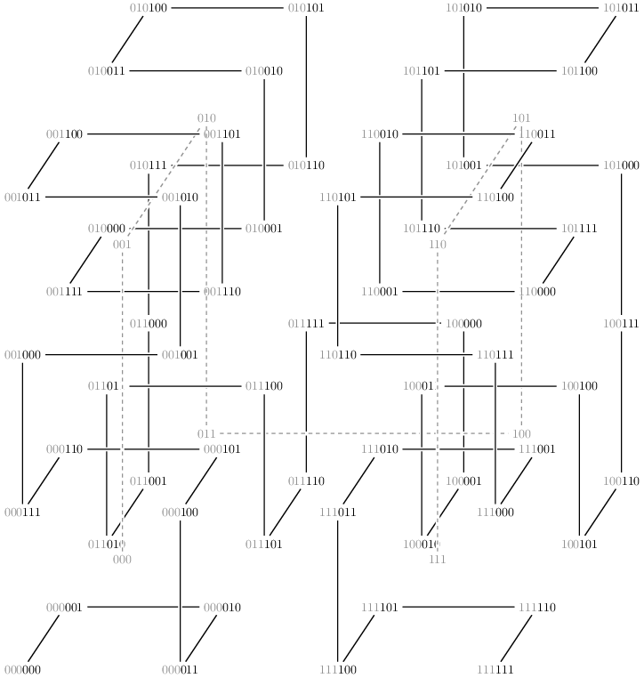
What about 3D?
All the curves I showed so far are nicely 2D, making them quite easy to compute and equally easy to show. But if you think back to the example I mentioned before, you might realise that we probably need 3D curves…
3D Morton curves are almost as easy to compute as their 2D counterparts; we simply need to interleave 3 bits for each level. For the Hilbert curve, things are (as usual) more complicated, since now 3D rotations are involved. You can spend a lot of time (and again, I did, so I know what I am writing about) trying to come up with the 3D equivalent of the maps above. If you are interested, you can find the lookup-table for 3D Hilbert curves I made in this source code file of my moving-mesh code Shadowfax (and if you happen to ever use it, please let me know, so I can feel good about having spent all that time on it).
And here is a picture I made about it for my PhD thesis:
Not so useful?
As you might have noticed, it is very easy to get carried away by space-filling curves. They seem very elegant and simple, but as often, this is just an illusion. However, I might have been too pessimistic about their usefulness.
Morton curves in particular are actually very useful. The fact that we need to compute Morton keys (albeit only level 1 keys) to locate the correct column in our Hilbert lookup-table is telling for their typical use: to order 2D or 3D space in a consistent way. But there is nothing really surprising in that: it seems very natural to count the points in a grid column by column from left to right (or row by row from top to bottom, or another permutation of these). Morton curve is just a fancy way of denoting this ordering.
The fact that the different levels in a Morton key tell you in which part of the box you are is also very useful, as this is exactly the information you need to build hierarchical structures like octrees or adaptive grids. I might tell you more about these in a future post.
But Hilbert curves, well, they are not so useful. Remember the example I gave above about the spatial domain-decomposition of points in space. And remember that I had to be quite vague in formulating the exact requirements of a good domain-decomposition (points have to be close in space). Well, turns out this is a fundamental issue with the way astronomers used to think about the decomposition of a computational problem across different computers… Spatial domain-decompositions do not actually give you the optimum decomposition for a problem, since they do not actually decompose what needs to be decomposed: the computations! Turns out computer science found a solution for this problem decades ago. And I promise I will write about this in a future post.
Professional astronomer.