I am currently exploring the limits of my code CMacIonize on an HPC system with a number of fat nodes (nodes with a large amount of RAM memory). The idea is to see how big a simulation I can run with the code on the available hardware (and within the available time). Part of this work consists of running large simulations for only a few steps, in order to gather as much as possible diagnostic information about the performance of the code: how long it takes to execute a single step, how long it takes to write an output file (a big worry for my simulations), how much memory the run requires… While doing this, I noticed that I had very little information about the overall balance of my simulations: I have very specific diagnostics to check the scaling of the code in various parts of the algorithm, but I do not have a good way of checking how the run time of various steps in the code compares.

To overcome this, I wrote a little helper class that makes it a lot easier to track the overall progress of a simulation and distinguish different steps in terms of performance. And then I wrote a Python script that can be used to visualise the output of this helper class. I will present both in this post.

The helper class

In order to track the progress of a simulation, I will use a time log, very similar to the MemoryLogger I mentioned briefly in a previous post. In essence, the time log is a simple list with entries that have a name and a start and end time. A new entry is created by calling a start function, and the entry is closed by calling an end function. At the end of the simulation, the entire list of entries is written to a large log file, ready to be analysed by the Python script.

There are a few issues that can arise with this. First of all, there is clearly a need to make sure that all entries that are created are also closed, as otherwise we might have entries without an end time. Secondly, the system with simple entries is not very good when you have various levels of entries. Suppose e.g. that your program consists of a few large steps, and you want to time each of these steps. Each step itself consists of a number of smaller substeps, and you also want to time these. If you add entries for both the steps and their substeps, then you will have nested start and end function calls, and your log file will contain overlapping entries. There will however not be any information that makes the link between the steps and their corresponding substeps, and your analysis script will somehow have to derive this information in order to disentangle overlapping intervals.

In order to deal with both issues, I decided to add two additional pieces of information to each log entry: the depth of that entry and its potential parent entry. The idea is to explicitly track the levels of entries. When the program starts, the root entry is created. This entry starts when the time log is created, and stops when the final time log file is written out. Every entry created between those two events is a level 1 entry, and its parent is the root entry. When a new entry is created within an open level 1 entry, that entry will be a level 2 entry with the open level 1 entry as parent, and so on. By looping through the final log and filtering out entries with a specific depth, we can choose to only analyse the large steps (level 1 entries), or to refine on smaller steps (higher level entries).

Now that we know which variables to track, it is straightforward to write a skeleton class representing a single log entry:

/**
 * @brief Single entry in the time log.
 */
class TimeLogEntry {
private:
  /*! @brief ID of the entry. */
  uint_fast32_t _ID;

  /*! @brief Label for the entry. */
  std::string _label;

  /*! @brief Start time stamp (in CPU cycles). */
  uint_fast64_t _start_time;

  /*! @brief End time stamp (in CPU cycles). */
  uint_fast64_t _end_time;

  /*! @brief Index of the parent entry. */
  uint_fast32_t _parent;

  /*! @brief Depth of the entry. */
  uint_fast32_t _depth;

public:
  ...
};

Note that, as explained before, I use a CPU cycle counter rather than an explicit time variable to measure time stamps. I also added a unique ID for each entry, to make sure we can flush the time log (write out some entries to a file to limit memory usage) and still have consistent links between entries. The public part of the class contains a trivial constructor and a number of setters and getters. Note that the constructor by default sets the parent and depth variables to 0.

The only non trivial member function of the TimeLogEntry class is the following:

  /**
   * @brief Close the entry.
   *
   * @param end_time End time for the entry (in CPU cycles).
   * @return Parent entry.
   */
  inline uint_fast32_t close(const uint_fast64_t end_time) {
    _end_time = end_time;
    return _parent;
  }

This function does two things: it sets the end time for the entry, and returns the index of the parent entry. We will use this function below.

The time log itself is represented by a second class called TimeLogger. The class has four member variables: a list (std::vector) with TimeLogEntry instances, a Timer to keep track of real execution time, an index for a currently active entry, and a counter for the last awarded entry ID. The latter stores the index of the last entry that was opened and not closed yet (i.e. the highest level entry that was not closed). The first part of the class definition looks like this:

/**
 * @brief Class to track time usage.
 */
class TimeLogger {
private:
  /*! @brief Time log. */
  std::vector< TimeLogEntry > _log;

  /*! @brief Timer. */
  Timer _timer;

  /*! @brief Active entry. */
  uint_fast32_t _active_entry;

  /*! @brief Last ID. */
  uint_fast32_t _last_ID;

  ...

Note that the Timer can be implemented in many ways (an example can be found here), and that it is not really important for our purposes. The only reason I use it is to be able to convert CPU cycles into real execution time.

The initialisation of the TimeLogger looks like this:

public:
  /**
   * @brief Constructor.
   *
   * Records the initial time stamp and starts the timer for normalisation.
   */
  inline TimeLogger() : _active_entry(0), _last_ID(0) {
    uint_fast64_t start_time;
    cpucycle_tick(start_time);
    _log.push_back(TimeLogEntry(0, "root", start_time));
    _timer.start();
  }

As explained in the comments, this constructor creates the root entry, sets it as the active entry, and starts the Timer.

To add new entries to the time log, we can use the following function:

  /**
   * @brief Start a new log entry with the given label.
   *
   * @param label Label for the entry.
   */
  inline void start(const std::string label) {
    uint_fast64_t start_time;
    cpucycle_tick(start_time);
    ++_last_ID;
    _log.push_back(TimeLogEntry(_last_ID, label, start_time, _active_entry,
                                _log[_active_entry].get_depth() + 1));
    _active_entry = _log.size() - 1;
  }

This code is very similar to the code to add the root entry, except that it now explicitly sets the parent for the new entry to the currently active entry, and the depth to the depth of the parent plus one. If the active entry is the root, then we created a level 1 entry. If the active entry has a higher level, then the new entry will be one level higher than that. Lastly, we set the active entry for the log to the newly created entry. Additional entries that are created before the new entry is closed, will automatically be children of the new entry.

To close an entry, we use the following function:

  /**
   * @brief Record the end of the given log entry.
   *
   * Note that this will only work if the last active entry has the same label.
   *
   * @param label Label for the entry.
   */
  inline void end(const std::string label) {
    uint_fast64_t end_time;
    cpucycle_tick(end_time);
    if (label.compare(_log[_active_entry].get_label()) != 0) {
      cmac_error("Trying to end time log entry that was not opened or that was "
                 "opened before the last entry was opened (label: \"%s\")!",
                 label.c_str());
    }
    _active_entry = _log[_active_entry].close(end_time);
  }

First, we record the end time for the entry. We then check if the label given to the entry matches the label of the active entry. If it does not, that means we are trying to close an entry that was opened before the last entry was opened, or an entry that was never opened at all (e.g. because we made a typo in the name). In this case we call the macro cmac_error, which will abort the program. Once we are sure the entry we are closing is the active entry, we set its end time and at the same time get the index for its parent entry, by using TimeLogEntry::close. The parent entry now becomes the active entry again. If the entry we just closed was a level 1 entry, this will be the root entry. If it was a higher level entry, then the active entry will correspond to the highest level unclosed entry.

The last method in the TimeLogger class is the one that takes care of the time log file output. It is by far the longest bit of code in the class, and is given below:

  /**
   * @brief Output the time log to the file with the given name.
   *
   * @param filename Output file name.
   * @param append Append to an existing log file?
   */
  inline void output(const std::string filename, const bool append = false) {
    if (_active_entry != 0) {
      cmac_error("Time log entries not properly closed!");
    }

    uint_fast64_t end_time;
    cpucycle_tick(end_time);
    _log[0].close(end_time);
    const double real_time = _timer.interval();
    const uint_fast64_t global_start_time = _log[0].get_start_time();
    const uint_fast64_t full_range = end_time - global_start_time;
    const double time_unit = real_time / full_range;

    std::ofstream ofile;
    if (append) {
      ofile.open(filename, std::ios_base::app);
    } else {
      ofile.open(filename, std::ios_base::trunc);
      ofile << "# entry id\tparent id\tdepth\tstart time (ticks)\tend time "
               "(ticks)\tstart time (s)\tend time (s)\tlabel\n";
    }
    for (uint_fast32_t i = 1; i < _log.size(); ++i) {
      TimeLogEntry &entry = _log[i];
      const double entry_start =
          (entry.get_start_time() - global_start_time) * time_unit;
      const double entry_end =
          (entry.get_end_time() - global_start_time) * time_unit;
      ofile << entry.get_ID() << "\t" << _log[entry.get_parent()].get_ID()
            << "\t" << entry.get_depth() << "\t" << entry.get_start_time()
            << "\t" << entry.get_end_time() << "\t" << entry_start << "\t"
            << entry_end << "\t" << entry.get_label() << "\n";
    }
    _log.resize(1);
  }

The method starts by checking that the active entry is the root, to make sure that all level 1 (or higher) entries are properly closed. If not, we abort the program. We then move on to recording the end time for the root entry. We also record the current execution time in seconds (_timer.interval()), and use that to compute a conversion factor from CPU cycles to execution time.

Next, we open the output file (either as a new file, or in append mode, based on the optional append boolean parameter). We then write out all relevant information for all entries except the root entry.

Finally, we flush the log by removing all entries except the root entry. This ensures that our time log does not grow indefinitely and prevents it from eating up all our memory.

Note that the output function can be called multiple times in a row. When it is called once at the start of the simulation without the append parameter (or with append = false), and afterwards with append = true, then it will produce a consistent chronological time line of the simulation that can be tracked while the program is still running.

The entire class can be seen at work in the following example code:

int main(int argc, char **argv) {

  TimeLogger time_logger;

  double value = 0.;

  time_logger.start("first loop");
  time_logger.start("first sub loop");
  for (uint_fast32_t i = 0; i < 1e6; ++i) {
    const double x = (0.5 + i);
    value += std::cos(2. * M_PI * x);
  }
  time_logger.end("first sub loop");
  time_logger.start("second sub loop");
  for (uint_fast32_t i = 0; i < 1e6; ++i) {
    const double x = (0.5 + i) * 0.1;
    value += std::sin(2. * M_PI * x);
  }
  time_logger.end("second sub loop");
  time_logger.end("first loop");

  time_logger.start("second loop");
  for (uint_fast32_t i = 0; i < 1e6; ++i) {
    const double x = (0.5 + i) * 0.1;
    value += std::sin(2. * M_PI * x);
  }
  time_logger.end("second loop");

  std::cout << "Result: " << value << std::endl;

  time_logger.output("test_timelogger.txt");

  return 0;
}

This will produce the following output file:

# entry id      parent id       depth   start time (ticks)      end time (ticks)        start time (s)  end time (s)    label
1       0       1       2566185721924657        2566185910480503        2.51901e-06     0.0819795       first loop
2       1       2       2566185721933154        2566185818487284        6.21319e-06     0.0419843       first sub loop
3       1       2       2566185818494423        2566185910480127        0.0419874       0.0819794       second sub loop
4       0       1       2566185910480871        2566186003258033        0.0819797       0.122316        second loop

The analysis script

To visualise the time log, I wrote a short Python script, the full version of which can be found here. I will not discuss the entire script (some of it deals with command line parameters or plot options), but I will highlight the relevant parts.

First, we need to read the time log file into a data array. Since the columns for the entries have mixed types, I use a custom data type in conjunction with numpy.loadtxt:

data = np.loadtxt(
    args.file,
    delimiter="\t",
    dtype={
        "names": ("id", "pid", "depth", "tic", "toc", "start", "end", "label"),
        "formats": ("u4", "u4", "u4", "u8", "u8", "f8", "f8", "S100"),
    },
)

The advantage of this approach is that the resulting array can be queried using the data type labels, e.g. data["label"] will return an array with all the labels.

To disentangle entries at different levels, I will plot entries with a different depth separately. First, I need to figure out the minimum and maximum depth among the entries:

mindepth = data["depth"].min()
maxdepth = data["depth"].max()

Note that the code in the full script is slightly different to allow for customisable limits.

The code to plot the entries as broken colour bars is below:

for depth in range(mindepth, maxdepth + 1):
    # select data for this depth
    idx = data["depth"] == depth

    # create a bar plot
    bar = [(line["start"], line["end"] - line["start"]) for line in data[idx]]
    colors = ["C{0}".format(i % 10) for i in range(len(data[idx]))]
    pl.broken_barh(bar, (depth - 0.4, 0.8), facecolors=colors, edgecolor="none")

pylab.broken_barh takes a list of tuples specifying the start and length of the individual bars. The vertical extends of the bar are chosen such that bars for different levels do not overlap. The only bit of real code magic is in the construction of the colors list: to distinguish neighbouring bars, we alternate through the list of 10 default matplotlib colours. We remove the edge colours to make sure very small bars are still visible and not hidden by the edge of neighbouring bars.

To add labels, we can add the following bit of code (within the same loop):

    # add labels
    labels = [line["label"] for line in data[idx]]
    for i in range(len(labels)):
        pl.text(
            bar[i][0] + 0.5 * bar[i][1],
            depth - 0.2 + 0.4 * (i % 2),
            labels[i],
            ha="center",
            bbox=dict(facecolor="white", alpha=0.9),
        )

This will first filter out the labels for this level, and will then plot them using pylab.text in the middle of the corresponding colour bar. To make sure neighbouring labels do not overlap too much (this will still depend a lot on the size of the underlying bar), we alternate between two vertical positions for the labels.

When used on the example time log above, the script produces the following image:

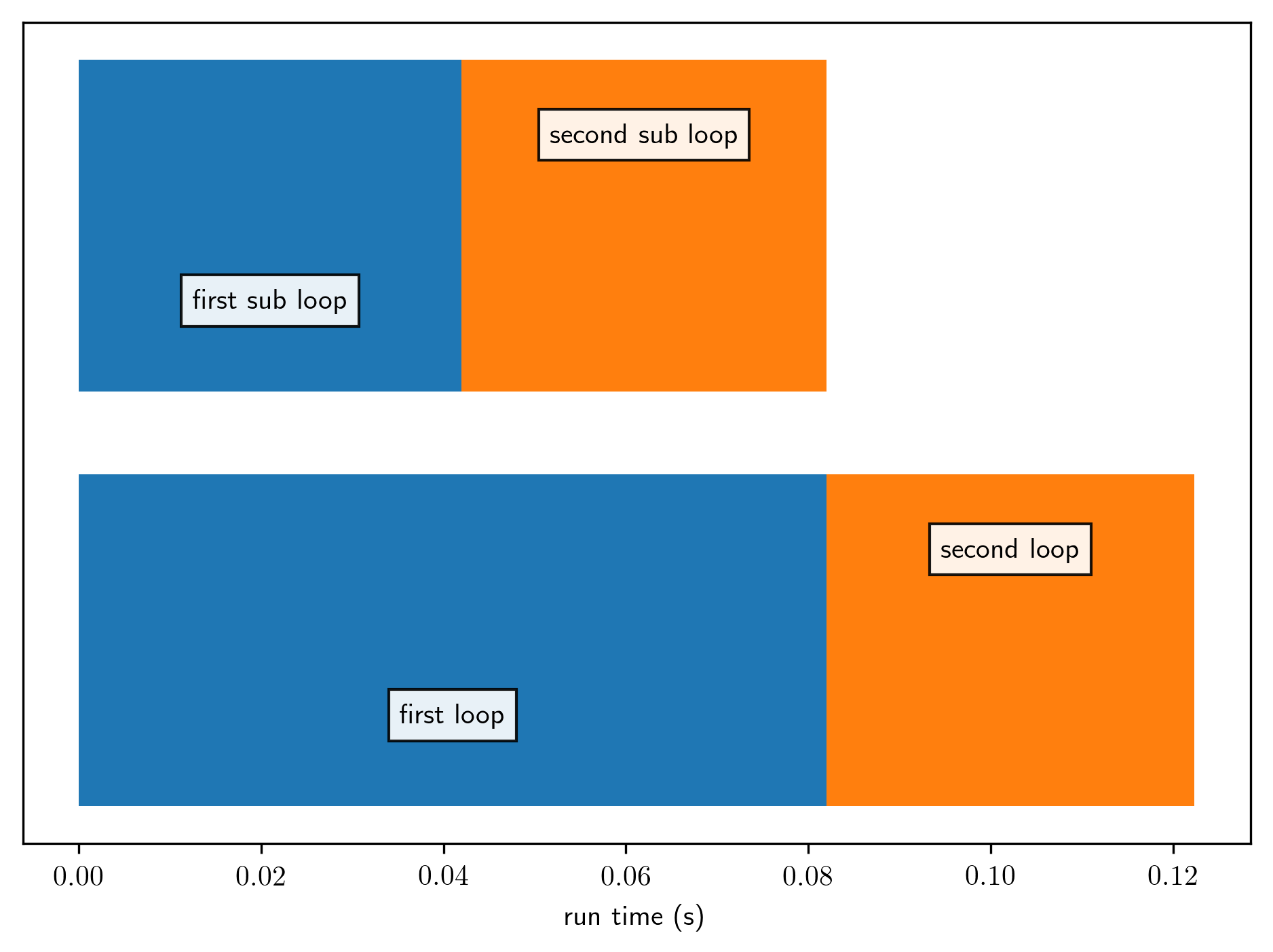
We can see that all three loops take roughly the same amount of time (which makes sense, given that they do roughly the same amount of work). The two sub loops for the first part are nicely plotted on top of the corresponding parent.

The full script also allows to select only specific parts of the time log. This can be easily done by filtering out elements in the data array before plotting it. For example:

pid = data[data["label"] == "first loop"
data = data[data["pid"] == pid[0]]

will only show the children of the first part of the time line. The presence of the parent ID column in the log file enables much more complicated queries than this to allow for better diagnostic information.

Not a profiler

Note that the helper class and analysis script provided here are a very poor version of a code profiler. If you want very detailed information about where in the code time is spent, you are better off using a real profiler (see a previous post. The code presented here has the advantage that it has very little overhead (if used wisely) compared to a real profiler, so that it can also be used during a high performance run and in situations where memory is valuable. I certainly have made good use of it this week.