I previously mentioned space-filling curves and their application in scientific computing, and concluded that post with the remark that space-filling curves are actually not the best solution if you want to distribute some large computational task over the separate nodes in a distributed memory parallel environment. In this post, I will show a more appropriate way to do this. And at the same time introduce another important mathematical concept: graph decomposition.

A short recap

Domain decomposition is the technical term for splitting up a large problem into smaller parts so that multiple processing units can work on it simultaneously. Suppose for example that you have a ridiculously large image ($1,000,000\times{}1,000,000$ pixels, a non-representative example of which is shown below) and you want to apply some sort of filter to each of its $1,000,000,000,000$ pixels.

If your filtering operation takes a millisecond per pixel, it would take a single processor unit almost $32$ years to finish the filter operation. Using all cores of a computer (let’s say there are $16$) reduces this to $2$ years. Using a supercomputer with $1,000$ of these computers (nodes) strung together reduces it to $17.5$ hours. Which is clearly a more acceptable time to wait.

In the case of the simple image filter (a clearly artificial case anyway) splitting up the image in $1,000$ pieces is the only thing required to work on it in parallel, and since operations on individual pixels are uncorrelated, the way these pieces match together (if they do) is not really important:

This changes when e.g. the filter operation does not only depend on the value of each pixel, but also on the value of its neighbouring pixels. After splitting up the image, it could happen that a node that is working on a specific pixel needs a neighbouring pixel that is stored on another node. In this case, the pixel information needs to be communicated from one node to another. This can only happen if we know where that pixel is located. Since this clearly also introduces an overhead (we need to do a communication that was not present in the original single threaded version of the filter), we clearly want to minimise the number of times this happens. In this case, the domain decomposition does not only need to split up the image, it also needs to (a) keep track of where the different pieces are relative w.r.t. each other, and (b) try to minimise the communication load caused by the decomposition.

Space-filling curves are a good way to decompose an image (or any other spatial domain) in an ordered way. They do however not directly address the second requirement for a good domain decomposition: they do not automatically minimise the number of communications. Despite this, they are still very often used for this purpose. The reason for this is that a space-filling curve (especially one with a constant separation length between successive points on the curve like the Hilbert curve) tends to (notice the choice of words) minimise the surface to volume ratio of the domains. Since the computational cost of a domain usually scales with the volume of the domain and its communication cost with its surface area, this leads to a decomposition with a small communication load.

This is however only true if the volume and surface area can be truthfully linked to respectively the computational cost and the communication cost, and if the factors linking both are fairly similar. Especially this last requirement is generally not satisfied: there is no reason why a domain that has a low volume to computation factor would also have a small surface area to communication factor or vice versa.

In other words, using a space-filling curve for your domain decomposition might provide very satisfactory results, but since it does not address the actual requirements for a true domain decomposition, it can also go terribly wrong. So it might be better to use a domain decomposition strategy that actually constructs a real domain decomposition.

Graphs

The image pixels in our example above each individually make up a computational unit, to which we can assign a number: the time it will take to apply the filter operation to that specific pixel. In our example, these numbers will be the same for each pixel, but this does not necessarily need to be the case.

Each pixel is linked to a number of neighbouring pixels (generally 4 or 8 - depending on whether or not we include the corners - but less for pixels near the border). If one of these links were to be broken (i.e. by putting the two pixels on separate node), this will lead to a communication. The corresponding communication overhead can also be measured (e.g. in time) and can be assigned as a number to the link that links both pixels.

We can now construct a diagram for the image in which each pixel constitutes a vertex, and its corresponding computational cost is its vertex weight. Neighbouring vertices are linked together with edges and the corresponding communication costs constitute an edge weight. The diagram itself is what we call a graph. It is a rigorously defined mathematical concept, with a lot of interesting properties (I’m sure) that I will mostly ignore. The graph for the example image is shown below.

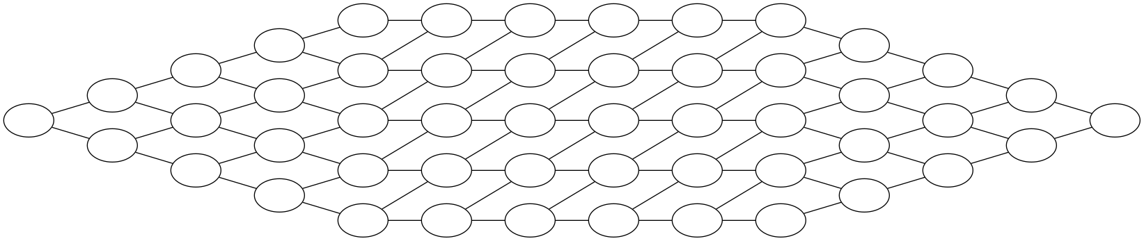
For our image, the corresponding graph is huge (it would actually take more memory to store it than it would take to store the actual image) and very structured. But graphs can be very complex and unstructured as well. Note also that in practice, we would never construct a graph for the whole image; the domain decomposition method below works just as well if we were to split up the image in a large enough number of small blocks (say $1,000\times{}1,000$ blocks of the same pixel size) and construct the graph for these blocks. As long as the individual blocks are small enough, the resulting domain decomposition will still be good.

Graph decomposition

Each decomposition of the image will automatically lead to a decomposition of the graph that represents the image. This decomposition of the graph will need to cut through some of the edges of the graph, and each of these cuts will cause a communication overhead. To minimise the total communication overhead, we have to make sure that the total accumulated edge cut cost is as low as possible.

The different parts of the decomposed graph will each contain a number of vertices, and each of these has an associated computational cost that represents the total workload for that part of the graph (or the associated part of the image). In order to obtain good scalability, we have to make sure the different parts of the image have an as equal as possible accumulated computational cost.

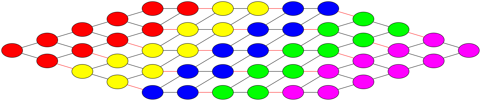
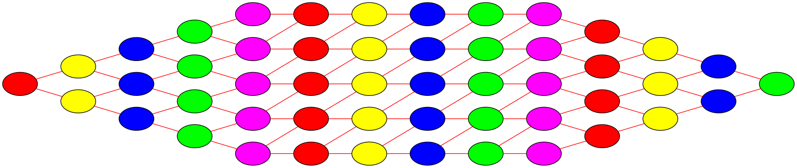
These two observations help us to rigorously define what we want to achieve for an ideal domain decomposition: we want to decompose the graph that represents the image and its connectivity (and corresponding communication overheads) so that each part of the decomposition has an accumulated vertex weight that is as close as possible to the decomposition average, and so that the accumulated edge cut caused by the decomposition is minimal. A good domain decomposition is hence the result of a mathematical optimisation problem, called a graph partitioning.

The graph partitioning for the example domain decompositions of our image example are shown below. The coloured edges are the edges that need to be cut to obtain the partitioning. Clearly, the second example is not a good decomposition.

Unfortunately, graph partitioning is part of a class of mathematical problems that are called NP-hard, meaning that, although an exact solution exists, it is generally not feasible to find it in any reasonable amount of time (and it is generally impossible to predict how long it would take). Hence, finding the best domain decomposition to speed up a computational problem is in itself a hard computational problem. That being said, there are some very good heuristic approximate methods that yield high quality graph partitions in a short (and predictable) amount of time.

METIS

Although there are many graph partitioning libraries that all do a reasonable job (Wikipedia lists 12 at the moment of writing), I will only mention the one that I use: METIS.

METIS is incredibly powerful, as it allows you to attach multiple weights to each vertex in the graph. This means that you can obtain domain decompositions that do not only distribute the computational workload evenly among the various nodes, but also distribute e.g. the memory load. Furthermore, it allows you to specify different target weights for the different pieces of the partition, which is useful for cases where some nodes have a different architecture than others (e.g. if half the nodes has 16 cores and the other half has 32).

ParMETIS (the MPI variant of METIS) does the graph partitioning in parallel and also has support for redistributing an existing decomposition. It will then not only recompute a more optimal decomposition, but will also factor in the computational cost required to redistribute the domains among the nodes.

Using METIS (or any of its variants) is relatively easy: the library is available on standard UNIX systems and can be included as any other library in your own programs. I will not go into too much detail here (maybe in a future post).

What about actual problems?

Thus far, I have illustrated graph decomposition using the fabricated example of a huge image. This can be easily extended to more concrete computational problems, like problems that involve a regular grid of cells. For less regular problems, it is still possible to construct a graph, although keeping track of the way the graph vertices map to actual problem units might be more tricky. In that case, it might be a good idea to still map to some kind of regular structure to do the decomposition, e.g. you can put N-body particles in boxes and decompose the boxes rather than the actual particles. As with the small image parts in our example, this will still yield good decompositions if the boxes are small compared to the overall simulation box size, so that each node always stores a significant amount of them. You can even out the particle load per node (if that is something you care about) by adding additional vertex weights for this.

A much more important (and tricky) part of using graph partitioning to obtain a domain decomposition is getting representative vertex and edge weights. As explained above, these weights should accurately represent the computational workload of the domain and the communication cost for cross-domain communication respectively. There are various options to get these weights, none of which are guaranteed to work.

First of all, you could explicitly count the number of operations to estimate the workload, and the data volume that needs to be communicated to estimate the communication cost. However, since actual execution time does not only consist of the CPU executing operations, but also involves the CPU retrieving the required data variables from memory and putting them back, this might not be the best estimate. In fact, many algorithms nowadays are memory-bound, meaning that the execution time largely depends on the time it takes to fetch variables from memory rather than on how fast the CPU executes operations on these variables. It is very hard to make accurate predictions for this, since these memory accesses depend on a lot of (unknown) factors, like the layout of your variables in memory, where the CPU is located (physically) w.r.t. the memory address that contains the variables, whether or not the same variable was used right before and is still stored in a faster cache register…

Another method to estimate weights is to measure the execution time for the different operations that are involved at run time. These measurements are likely a better estimate for the actual execution time, as they naturally factor in the things mentioned above. However, even these measurements are not necessarily representative for the actual computational cost, as CPUs do not always operate at the same efficiency. For communications, execution time depends a lot on the MPI library you are using for the communication. Experience learns that some MPI implementations can have wildly varying communication costs.

So in practice, the best way to find good cost estimates is by simply trying out various things and observing how different estimates behave for your specific problem. Depending on the nature of the problem, it might be easier to come up with some easy to compute heuristic estimate that does a better job at balancing the computation than any of the methods mentioned above. And even then, there is no guarantee that a method that performs well on one cluster with one specific MPI implementation also works well on another cluster with another MPI implementation. The best advice is to make sure you have appropriate ways to measure the behaviour of your code, figure out what causes bad behaviour and quantify the impact of various cost estimates, so that it is easy to adapt to a specific situation.