NOTE: the expression computed in this post is subtly wrong and has been corrected in a more recent post.

And now for something completely different. I recently encountered an interesting geometry problem during my work on light scattering off non-spherical particles, and this problem led to an interesting derivation that I would like to document, mostly for myself.

The problem is this. When light scatters off a spherical particle, part of the light will be absorbed. We can compute the amount of light that is absorbed by a particle with a given composition (there are various techniques to do this), and if we divide this by the average surface area of the particle that is exposed (which will be bigger for larger particles), we end up with an absorption coefficient that encodes how efficiently particles of that given composition absorb light.

The project I am currently working on requires me to generalise this technique to non-spherical particles of a specific type: spheroids. Spheroids are 3D generalisations of 2D ellipses: the easiest way to think about them is by imagining a sphere that is either stretched in one direction (in which case we call the spheroid prolate) or flattened in a direction (this is an oblate spheroid). Mathematically, the surface of a spheroid is described by the following equation:

i.e. it consists of all points in space with coordinates $(x,y,z)$ for which the above equation holds. The parameters $a$ and $b$ are called the semi-major and semi-minor axes of the spheroid, depending on which one is the largest. For prolate spheroids, this will be $b$, while for oblate spheroids, $a$ is the largest and hence the semi-major axis. The axis ratio $d=a/b$ is also frequently used to distinguish between the two types of spheroids; $d>1$ is an oblate spheroid and $1>d$ a prolate spheroid. Spheroids with $d=1$ have $a=b$, in which case the whole equation reduces to that of a sphere. The semi-major and semi-minor axis are in this case both equal to the radius $r$ of that sphere.

The technique to compute the scattering and absorption for spheroidal particles is quite complicated and not very relevant for this post, so I will simply mention that it exists and works (I didn’t invent this technique myself; some very clever people in the 70s did this). Let’s instead get back to the problem I wanted to introduce. It turns out that, if you want to compute the absorption coefficient, you need to divide whatever absorption cross section (the physical equivalent of an absorption efficiency for a given particle) by the average surface area of the particle to end up with a quantity that does not depend on the size of the particle anymore. If your absorbing particle is a sphere with radius $r$, then this average surface area is simply the surface area of the projection of that sphere you see in any direction: a simple disc with radius $r$ and hence surface area $\pi{}r^2$.

For spheroids, this is no longer true; the projection of a spheroid is only a disc if you look at it along its symmetry axis (the $z$ axis in the equation). From any other viewing direction, the projection will be a more general ellipse, the properties of which depend on the viewing direction. However, in the relevant scientific literature, people usually choose to ignore this fact, and instead still use a surface area given by $\pi{}r_V^2$, where $r_V$ is a so-called equivalent volume sphere radius, i.e. the radius of a sphere that has the same volume as the spheroid. Since the volume of a spheroid is given by $\frac{4\pi{}}{3}a^2b$, this radius is given by

This finally brings us to the problem I encountered. Turns out that, if you compute absorption coefficients for spheroidal particles using the exposed surface area based on $r_V$, these absorption coefficients are systematically higher than what you get for spherical particles with the same radius, irrespective of whether the spheroidal particles are oblate or prolate. This is a bit weird, as you would not expect the shape of a particle to have a significant impact on how much radiation the particle can absorb (it might affect how this absorption differs for different infalling directions; that is why we are interested in these particles in the first place), unless of course the particle has more opportunity to interact with the radiation, e.g. because the exposed surface area of the particle is significantly larger than our $r_V$ based guess.

So the question I wanted to answer is the following: is there a better way to estimate how much surface area is exposed for a spheroidal particle with axis ratio $d$ and equivalent volume sphere radius $r_V$, and can this explain the systematically higher absorption coefficients I find?

Solving the problem

Solving the problem in essence boils down to computing what I call the average active surface area: the surface area of the spheroidal particle as seen in projection for a specific viewing angle, averaged out over all possible viewing angles. If we use the same coordinate frame that we used for the equation of the spheroid above (where the $z$ axis is aligned with the particle symmetry axis), and we call the angle between the infalling direction and the $z$ axis the zenith angle $\theta{}$ and the angle between the (arbitrarily chosen) $x$ axis and the projection of the infalling direction in the $xy$ plane the azimuth angle $\phi{}$, then we can call the projected surface area for that infalling direction $A(\theta{},\phi{})$. The average active surface area can then be computed using the following equation:

We simply need to find an expression for $A(\theta{},\phi{})$. This is not so simple, as we will see below.

Azimuth dependence and symmetry

Before trying to derive this expression, it is worth thinking about the problem some more. The question we need to ask is: does this expression really depend on two angles? It makes sense that the projected surface area depends on the zenith angle $\theta{}$, as a different value of $\theta{}$ means you get a different projected value for the vertical axis of the spheroid, and this will change the shape of the projected ellipse. The same does not hold for the azimuth angle $\phi{}$: if this angle changes, you will see different projected values for the axes along $x$ and $y$, but since the choice of a particular $x$ and $y$ axis itself is arbitrary within the $xy$ plane, these projections will always be the same. Or in other words, because the spheroid has the same semi-minor/major axis for both $x$ and $y$, the projected ellipse will always have a semi-minor/major axis with size $a$, independent of the azimuth angle $\phi{}$.

This is a good example of symmetry: the equation for the spheroid and its projection does not change if we rotate the entire spheroid around its symmetry axis $z$ with an arbitrary angle. It also means that our exposed surface area will only depend on $\theta{}$, so that we can already compute part of the integral above:

Even better: we already now that the exposed surface area will be given by

where the only thing left to find is the second axis of the projected ellipse, $c(\theta{})$.

Projected ellipse

A first naive idea you might have is that the second axis of the ellipse is always a projection of the second axis of the spheroid, $b$. In this case this projection probably only depends on $\theta{}$, and things become very easy to solve. Unfortunately, this is not true. While, depending on the exact shape of the spheroid, there are directions $\theta{}$ from which you effectively see a projection of the axis $b$ (e.g. $\theta{}=\pi{}/2$), this is definitely not true for some other angles. $\theta{}=0$ e.g. corresponds to the case where you see the spheroid along its symmetry axis, in which case the second axis is $a$, not a projection of $b$. In other words, the second axis needs to be a combination of both $a$ and $b$ that somehow naturally transitions between these two extreme projection cases.

The axis length we are after is essentially the line segment enclosed within two projection lines that are parallel to the line of the incoming direction $\theta{}$, and that are tangent lines to the surface of the spheroid, which is an ellipse with axes $a$ and $b$ if we draw its cross section. To determine the unknown axis length $c(\theta{})$, we need to determine the coordinates of the tangent points where these tangent lines touch the ellipse, and then determine half the distance between these two points.

To get the slope of the tangent lines to a general curve with a known equation, we need to compute its derivative. To do this, we first rewrite the equation of the ellipse,

in terms of an actual function of $x$:

As you can see, we actually end up with two functions, since the square root has two roots (corresponding to the upper and lower half of the ellipse).

The derivative of this function w.r.t. $x$ is

We somehow have to relate this equation (these equations) with the infalling direction and the angle $\theta{}$. The requirement that the tangent lines are parallel to a line through the centre that makes an angle $\theta{}$ with the $y$ axis, just means that the slopes we found above should be the same as the slope of this reference line, which is $1/\tan(\theta{})$. By equating both expressions for the slope, we can determine the $x$ coordinates for which this is true; these are the $x$ coordinates of the tangent points:

To find the corresponding $y$ coordinates, we can plug these values into the equation of the ellipse:

There is some ambiguity in how we need to select the signs for these $x$ and $y$ values, but for our purpose that is not very relevant, since we are only interested in the distance $D$ between these points. Generally, the distance between two points with coordinates $(x_1,y_1)$ and $(x_2,y_2)$ is

In this case, only the positive root is used, since distances are always positive. In our specific case, we will - irrespective of the sign - always have combinations of positive and negative $x$ and $y$ coordinates, and the squares will automatically eliminate the resulting sign. We end up with

We can check that this expression makes sense by plugging in the values for $\theta{}$ for which we know what $c(\theta{})$ should be. For $\theta{} = 0$, we find $c(\theta{}) = a$. For $\theta{}=\pi{}/2$ we have a problem however, as $\tan(\pi{}/2)$ is divergent. The mathematically correct way to handle this would be to do some kind of limiting procedure, but we can actually solve this problem in a more elegant way: the $\cos(\theta{})$ in the denominator of $\tan(\theta{})$ that causes the divergent behaviour appears both in the nominator and the denominator in the $c(\theta{})$ expression, so we can simply divide it out:

This expression behaves nicely for all values of $\theta{}$, and for $\theta{}=\pi{}/2$ we find $c(\theta{})=b$, as expected.

There is one additional change we can make to make this equation more practical: we can replace the explicit non-linear dependence on both axis lengths $a$ and $b$ with a linear dependence on one of them, and an explicit dependence on the more general axis ratio, $d=a/b$:

Back to the integral

If we substitute the expression for $c(\theta{})$ we found above in the integral that we need to compute, we find

After making an obvious change of integration variable, we can turn this into the following expression:

Since we want to know how different this value is from the fiducial surface area $A=\pi{}r_V^2 = \pi{} a^2 d^{-2/3}$, we are actually interested in the ratio $R = \langle{}A\rangle{}/A$:

which, conveniently and unsurprisingly, only depends on the axis ratio $d$.

We can again do some sensibility checks on this expression. We know that for $d=1$ (a spherical particle) $R=1$, and this is also what we get if we plug this into the expression.

Unfortunately, I don’t think the integral in the above expression can be analytically solved for general values of $d$. It is however very easy to compute this integral numerically and plot the value of R:

import numpy as np
import scipy.integrate as integ
import matplotlib
matplotlib.use("Agg")
import matplotlib.pyplot as pl

pl.rcParams["text.usetex"] = True

def integrand(x, d4m1, d2m1):
  return np.sqrt((d4m1*x**2 + 1.) / (d2m1 * x**2 + 1.))

drange = np.linspace(0.5, 2., 100)
frange = np.zeros(drange.shape)
for i in range(len(drange)):
  d = drange[i]
  d4m1 = d**4 - 1.
  d2m1 = d**2 - 1.

  frange[i] = \
    0.5 * integ.quad(integrand, -1., 1., args=(d4m1,d2m1))[0] / np.cbrt(d)

pl.plot(drange, frange)

pl.xlabel("$d = a/b$")
pl.ylabel("$R = \\langle{}A\\rangle{}/A$")

pl.tight_layout()
pl.savefig("equal_active_area.png", dpi = 300)

The result is shown below:

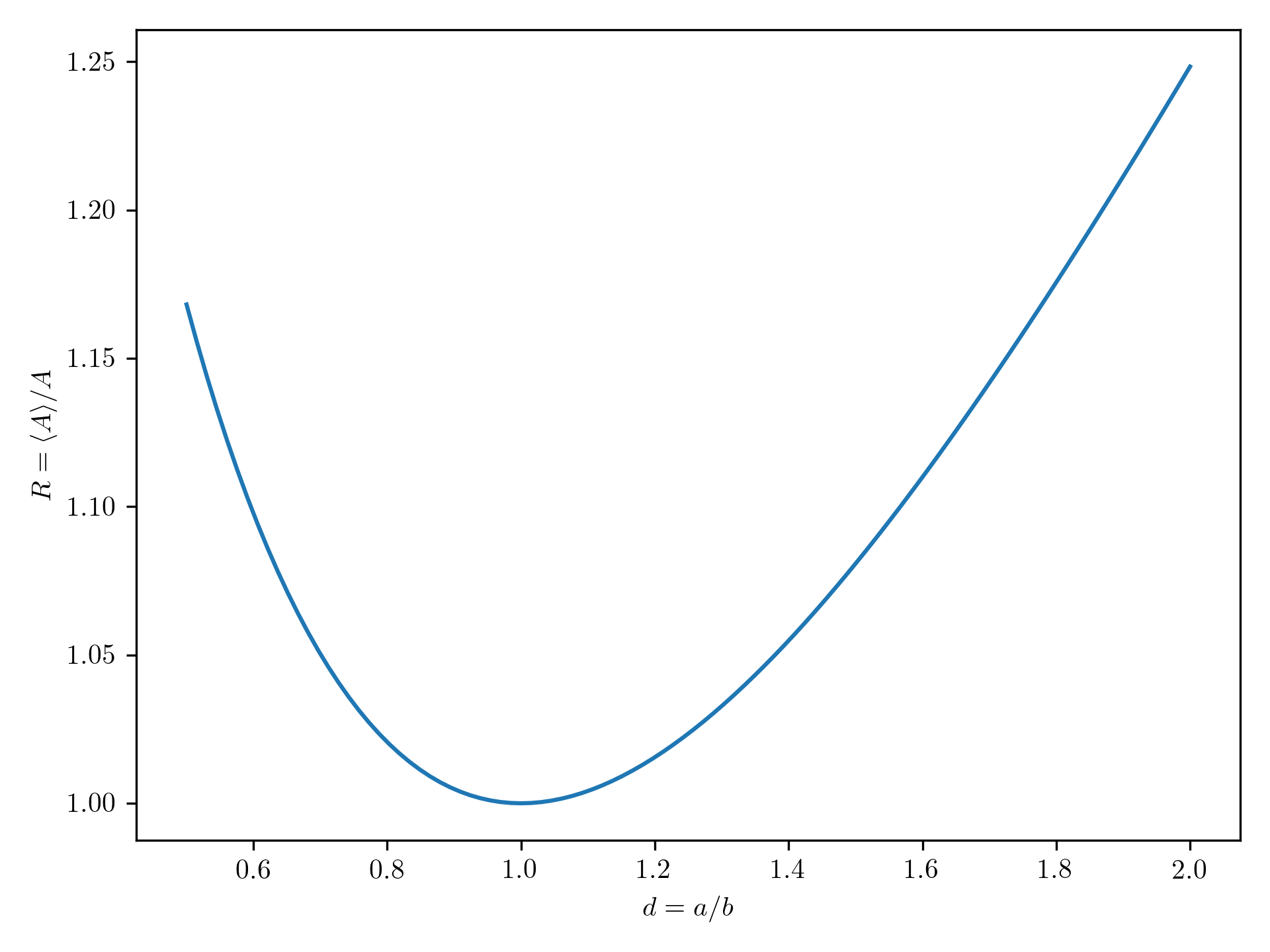
As it turns out, the ratio $R$ is indeed higher than $1$ for any spheroid with $d\neq{}0$, so the higher absorption coefficients that we find can be attributed to a change in $\langle{}A\rangle{}$.