In a previous post, I computed the average active cross section for a spheroidal particle with axis ratio $d=a/b$. It has since come to my attention that the expression I computed in that post is in fact wrong, so I thought it would be fair to post a correction.

I first discovered that this expression is wrong by reading a book from the 80s (the original version of this book dates back to the 50s). In that book, it is stated that the average active cross section of any convex particle (including spheroids) is simply $1/4$ of the surface area of that particle. Turns out this is actually a mathematical theorem that dates back all the way to Cauchy in the 1800s.

The surface area of a spheroidal particle with axis ratio $d$ and long axis $a$ is given by

$$S(d) = 2 \pi{} a^2 \left(1 + \frac{1}{d \sqrt{1-d^2}}\arcsin{\sqrt{1-d^2}}\right)$$

for $1 > d$ (prolate spheroid), and

$$S(d) = 2 \pi{} a^2 \left(1 + \frac{1}{d \sqrt{d^2-1}}{\rm{}arcsinh}{\sqrt{d^2-1}}\right)$$

for $d > 1$ (oblate spheroid).

The resulting average active cross section according to Cauchy is shown below, in blue. The orange line is the expression found in my previous post, which is clearly not the same…

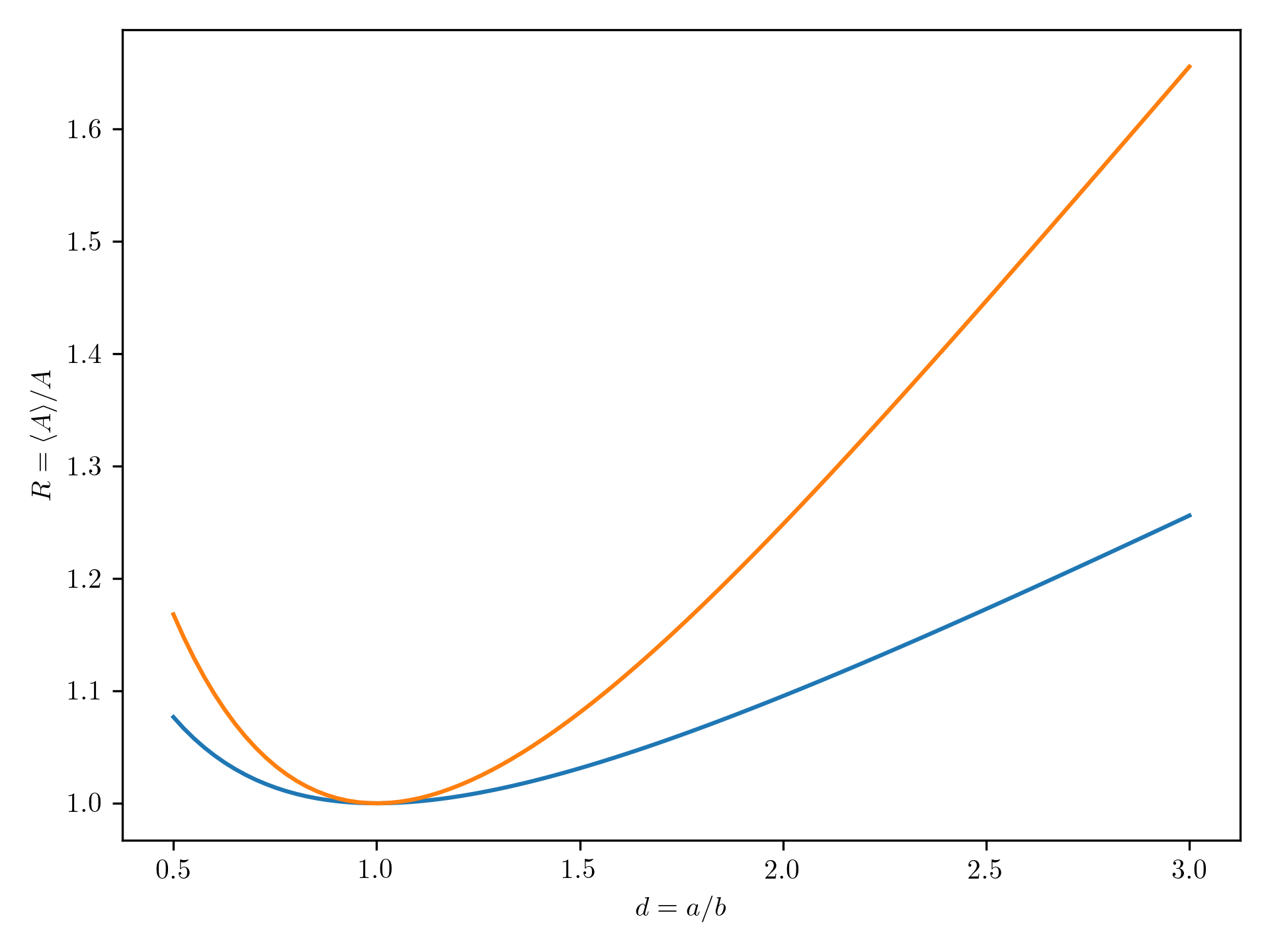
So where did I go wrong?

Remember that the average active area is computed using an integral, by averaging out the projected cross section for a given direction $\theta{}$ over all directions. The projected cross section for each direction is the surface area of an ellipse with one axis equal to $a$, while the other axis length depends on the angle. To compute this variable axis length, I first looked at the cross section of the spheroid in the plane of the incoming direction, which is an ellipse with axes $a$ and $b$. The projection of this ellipse perpendicular to the viewing direction is a line segment, and the length of this line segment is equal to twice the axis length we are looking for.

This is depicted in the image below:

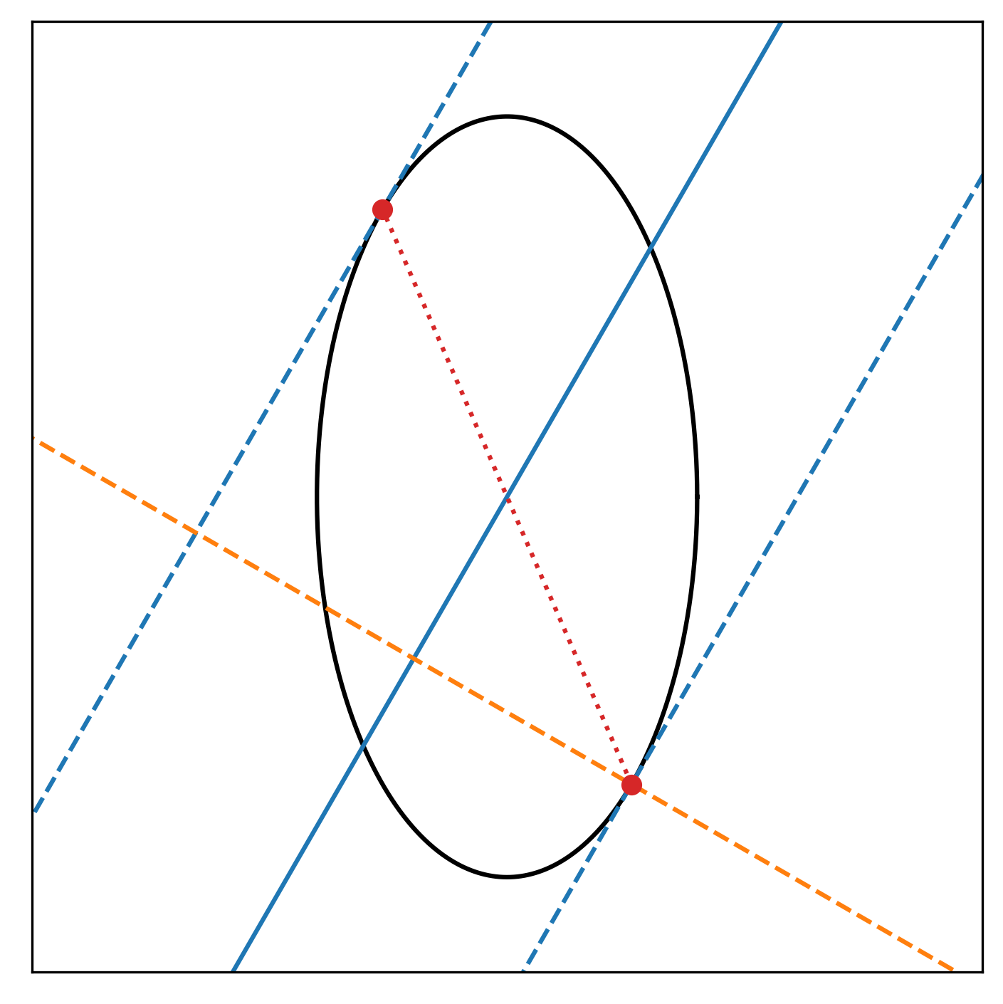
To find the line segment in question, we first need to find out what the tangent lines to the ellipse are (blue dashed lines). These are parallel to the viewing line (solid blue line), and go through points on the ellipse (red points). The coordinates of the red points can be found using some basic analytic geometry, as I did in my old post.

The error I made was in the next step: finding the length of the projected line segment. In my old post, I took this length to be the length of the segment in between the red points (red dotted line). However, as can be seen from the figure, the red line segment is not actually perpendicular to the viewing line, so this is incorrect. In fact, it is only correct if the ellipse were a circle, which explains why the old expression is correct for the case $d=1$.

Instead of using the red line segment, what we need to determine is the length of the line segment along the orange dashed line and in between the two blue dashed lines. This is a lot harder than the simple distance expression in the old post, so I had to revert to some symbolic algebra using the Python package sympy to achieve this. I won’t go into details here, as that would require me to write down too many equations. Without equations, what you need to do is (a) construct the orange line as the line perpendicular to the bottom blue line and going through the bottom red point, (b) determine the intersection point of the orange line with the top blue line, (c) compute the distance between bottom red point and this intersection point.

Assuming the coordinates of the red points are given by $(x_1, y_1)$ and $(-x_1, -y_1)$, the distance expression in my old post, which read

$$c(\theta{}) = \frac{1}{2}\sqrt{(2x_1)^2 + (2y_1)^2}$$

needs to be changed to

$$c(\theta{}) = \frac{\sqrt{2}}{2} \sqrt{x_1^2 + y_1^2 + (x_1^2-y_1^2)\cos{2\theta{}} - 2x_1y_1\sin{2\theta{}}}.$$

When we substitute the expressions for $x_1$ and $y_1$ found in my old post, this leads to the following expression for the unknown axis length:

$$c(\theta{}) = b\sqrt{(d^2-1)\cos^2{\theta{}} + 1}.$$

This expression is actually more compact than the old expression. As before, plugging in $\theta{}=0$ yields $c(\theta{})=a$, while plugging in $\theta{}=\pi{}/2$ yields $c(\theta{})=b$, as expected.

Using this new expression, I find the following plot for the average active cross section as a function of axis ratio:

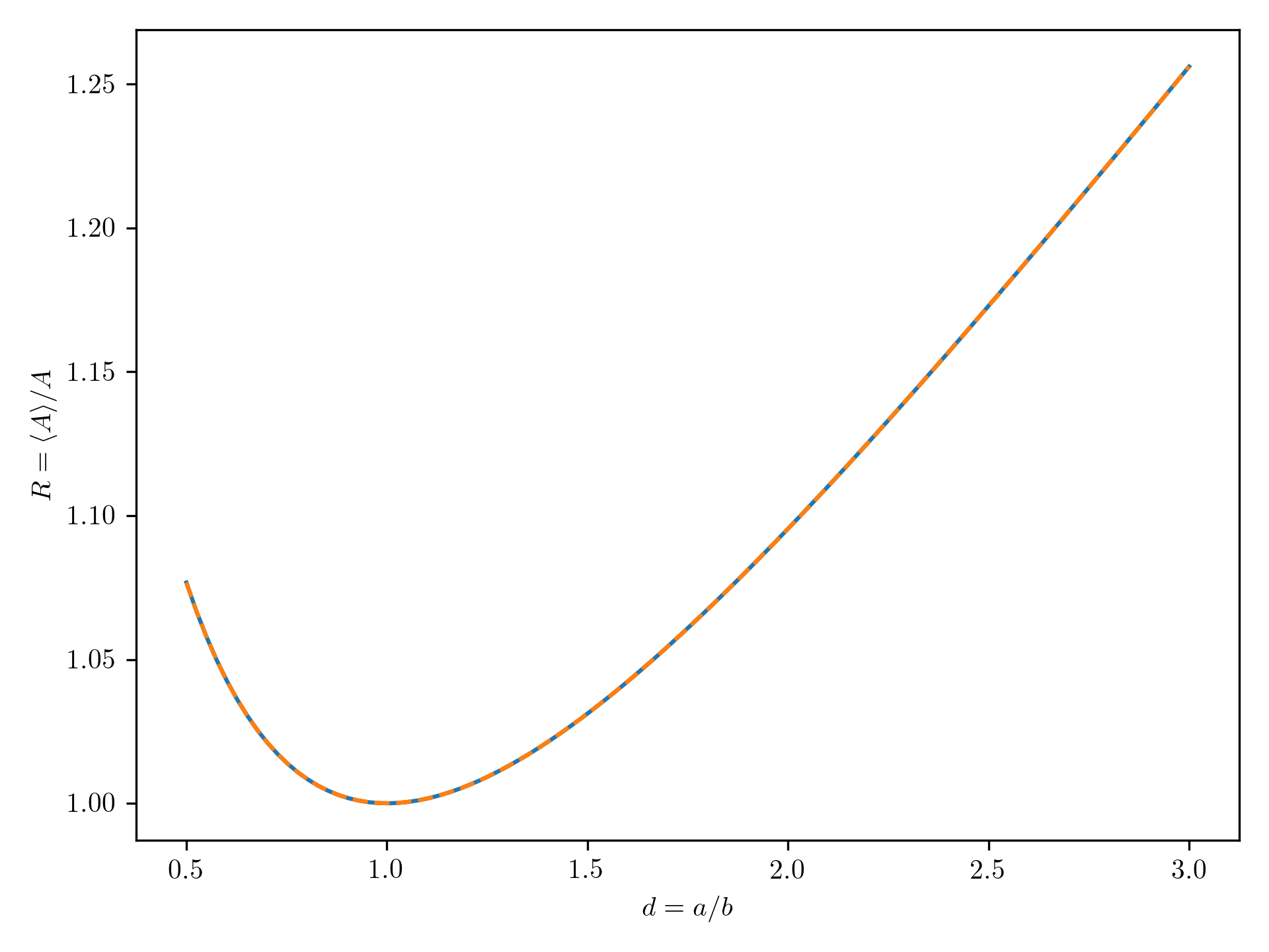
Both curves are now indistinguishable.